‘Ready, Integrate, Fire!’ Part 2: Simulating a simple neuronal model

20 minute read

Published: February 14, 2018

This Jupyter notebook will simulate a leaky integrate-and-fire neuron model with static input current using Numpy. We will also verify the formula for theoretical firing rate we derived in the last blog post.

This is a direct Python translation (with a slight modification) of the Matlab code found in this tutorial paper created by the Goldman Lab at UC Davis.

In my last blog post, I presented the Leaky Integrate-and-Fire Model, where a neuron is modelled as a leaky capacitor with membrane resistance $R_m$ , time constant $\tau_m$ , and resting potential $E_L$ . Below the threshold value $V_{th}$ , the equation for the voltage $V(t)$ of this neuron when it receives a current injection $I_e$ is given by:

$\tau_m \dfrac{dV}{dt} = E_L - V + R_mI_e. \hspace{1 cm} (Eq 1)$

To generate action potentials, this equation is augmented by the golden rule: whenever $V$ reaches the threshold value $V_{th}$ , an action potential is reset to $V_{reset}$ .

We solved Eq1 analytically, and if we know the value $V(t_0)$ of the neuron’s membrane potential at the reference point $t_0$ , the solution is as follows:

$V(t) = E_L + R_mI_e + [V(t_0) - E_L - R_mI_e]e^{-(t-t_0)/\tau_m}. \hspace{1 cm} (Eq 2)$

Setting $t_0$ equal to the current time in a simulation and $t$ equal to the time a single time-step $\Delta t$ later results to the following one-time-step update rule we will use for simulating the LIF neuron:

$V(t+\Delta t) = E_L + R_mI_e(t) + [V(t) - E_L - R_mI_e(t)]e^{-\Delta t/\tau_m}. \hspace{1 cm} (Eq 3)$

For concreteness of our simulation, we will use parameter values $\tau_m = 10$ ms, $E_L = -70$ mV and $R_m = 10$ $M\Omega$ . We will assume that, initially at time $t=0, V=E_L$ .

To model the spiking of the LIF neuron when it reaches threshold, we will assume that when the membrane potential reaches $V_{th} = -55$ mV, the neuron fires a spike and then resets its membrane potential to $V_{reset} = -75$ mV.

We will inject various levels of current $I_e$ into the model neuron, and to calculate the experimental firing rate, we will count the number of action potentials in a fixed amount of time. For this simulation, we will assume that the neuron receives a static current pulse of magnitude $I_0$ for 300 ms beginning at time $t_{pulse} = 100$ ms and plot several representative values of $I_e$ that produce firing rates between 1 and 100 Hz. We will run our simulations for 500ms total (i.e. 100 ms with $I_e$ =0; 300 ms with $I_e=I_0 >0$ ; and another 100 ms with $I_e = 0$ . We will discretize Eq1 and run our simulation with a time step $dt = 0.1$ ms.

Let’s start coding!

Part 1: Model the subthreshold voltage dynamics

We will add the spiking rule in the latter part of this notebook. For the first part, we will need to model the subthreshold voltage dynamics governed by Eq 1. We’ll follow the tutorial’s general overall strategy to break our code into the following sections:

Define the parameters in the model.
Define the vectors that will hold our final results such as the time, voltage, and current; and assign their initial values corresponding to $t=0$ .
Integrate the equation(s) of the model to obtain the values of te above vectors at later times by updating at the previous time step with the update rule.
Make good plots of our results.

Step 1: Import Relevant Packages

We will need only two libraries: Numpy and Matplotlib. These two packages are useful for scientific computing and data visualization, respectively.

import numpy as np
import matplotlib.pyplot as plt

Step 2: Define Parameters

We’ll define the model parameters as discussed above. In general, it is helpful to have a section of your code dedicated to assigning values to all model parameters (the variables that have fixed values throughout the entire simulation). It is also a good programming style to make a comment describing each parameter and noting its units. This will be very valuable in spotting errors once they occur.

dt = 0.1 #time step [ms]
t_end = 500 #total time of run [ms]
t_StimStart = 100 #time to start injecting current [ms]
t_StimEnd = 400 #time to end injecting current [ms]
E_L = -70 #resting membrane potential [mV]
V_th = -55 #spike threshold [mV]
V_reset = -75 #value to reset voltage to after a spike [mV]
V_spike = 20 #value to draw a spike to, when cell spikes [mV]
R_m = 10 #membrane resistance [MOhm]
tau = 10 #membrane time constant [ms]

Step 3: Define Initial Values and Vectors to Hold Results

We need to set up the initial conditions for the run (i.e. specify what the values of the relevant variables will be at time $t=0$ ) and to define and initialize variables (often vectors) that will hold all of the information we eventually might want to plot or use for other purposes. For our simulation, we’ll be plotting voltage vs. time so let’s define a time vector running from $t=0$ to $t=t_{end}$ in time steps of size $dt$ ; in a corresponding voltage vector that will hold the voltage at each of these times. Programming tip: put “_vect” on the end of the names of all vector variables to help you distinguish them from the scalars.

t_vect = np.arange(0,t_end+dt,dt) #will hold vector of times
V_vect = np.zeros((len(t_vect),)) #initialize the voltage vector
V_vect[0] = E_L #value of V at t = 0
I_e_vect = np.zeros((len(t_vect),)) #injected current [nA]
I_Stim = 1 #magnitude of pulse of injected current [nA]
I_e_vect[np.int(t_StimStart/dt):np.int(t_StimEnd/dt)+1] = I_Stim*np.ones((np.int((t_StimEnd-t_StimStart)/dt)+1,))

Note that we want that at time $t=0$ , $V=E_L$ , so we set the first element of V to this value. We also defined the current injected at all times as $I_{e-vect}$ . Sinec we want to start simulating at time $t_{StimStart}=100$ ms and end at time $t_{StimEnd} = 400$ ms, we also set the elements of $I_{e-vect}=I_{StimPulse}$ between 100 and 400 ms where $I_{StimPulse}$ is the amplitude of the injected current during the simulation. We have set this value to 1 nA.

Step 4: Write Leaky Integrate-and-Fire Neuron Model

We are now ready to integrate Eq1. To do this, we need to implement the update rule (Eq 3) using a for loop that iterates over the values of $t$ .

for i in range(1,np.int(t_end/dt)+1): #loop through values of t in steps of dt ms, start with t=1 since we already defined V at t=0
	V_vect[i] = E_L + I_e_vect[i]*R_m + (V_vect[i-1] - E_L - I_e_vect[i]*R_m)*np.exp(-dt/tau)

Step 5: Make Plots

Now we are ready to plot the subthreshold dynamics of our leaky integrate-and-fire neuron.

plt.plot(t_vect, V_vect)
plt.title('Voltage vs. time')
plt.xlabel('Time in ms')
plt.ylabel('Voltage in mV')
plt.show()

png

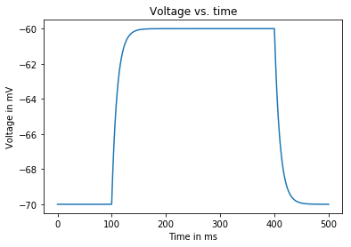
As can be seen in the above graph, the voltage (in mV) should rise exponentially towards -60 mV starting at $t=100,$ then decay back exponentially at $t=400$ (both rise and decay with time constants at $\tau =10$ ms).

Feel free to try out other values of $I_{stim}$ on your own to get a feeling for how big voltage change you get for different values of $I_{stim}$ .

Part 2: Add the spiking to the model and calculate the firing rate

I hope you noticed that no matter how large you made $I_{Stim}$ , our current model did not spike. We need to add the code to make the neuron spike and then reset each time its voltage reaches the threshold value $V_{th}$ . We’ll do this by modifying Steps 3-5 of our previous model.

Step 3 (v2): Define Initial Values and Vectors to Hold Results

We have to assign a new vector $V_{plot-vect}$ which replaces the first time point after threshold by a high spike point at voltage $V=V_{spike}=20$ mV. This value is arbitrary as the LIF model never really assigns a specic voltafe above $V_{th}$ . Every time threshold is reached, it immediately rests the voltage to $V_{reset}$ , which is our signal that a spike occurred at this time if we are trying to count the number of spikes.

t_vect = np.arange(0,t_end+dt,dt) #will hold vector of times
V_vect = np.zeros((len(t_vect),)) #initialize the voltage vector
V_plot_vect = np.zeros((len(t_vect),)) #pretty version of V_vect to be plotted that displays a spike whenever voltage reaches threshold
V_vect[0] = E_L #value of V at t = 0
V_plot_vect[0] = V_vect[0] #if no spike, then just plot the actual voltage V
I_e_vect = np.zeros((len(t_vect),)) #injected current [nA]
I_Stim = 1.55 #magnitude of pulse of injected current [nA]
I_e_vect[np.int(t_StimStart/dt):np.int(t_StimEnd/dt)+1] = I_Stim*np.ones((np.int((t_StimEnd-t_StimStart)/dt)+1,))

Step 4 (v2): Write Leaky Integrate-and-Fire Neuron Model

We add the spiking rule to this step and modify the integration loop for reflect this in our plots and results.

for i in range(1,np.int(t_end/dt)+1): #loop through values of t in steps of dt ms, start with t=1 since we already defined V at t=0
	V_vect[i] = E_L + I_e_vect[i]*R_m + (V_vect[i-1] - E_L - I_e_vect[i]*R_m)*np.exp(-dt/tau)
	if (V_vect[i] > V_th): #neuron spiked
		V_vect[i] = V_reset #set voltage back to V_reset
		V_plot_vect[i] = V_spike #set vector that will be plotted to show a spike here
	else: #voltage didn't cross threshold so neuron does not spike
		V_plot_vect[i] = V_vect[i] #plot actual voltage

Step 5 (v2): Make Plots

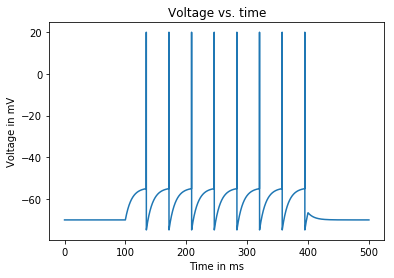
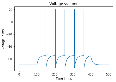
We also need to change our plotting code to plot $V_{plot-vect}$ rather than $V_{vect}$ . We should see 8 beutiful spikes like the one below:

plt.plot(t_vect, V_plot_vect)
plt.title('Voltage vs. time')
plt.xlabel('Time in ms')
plt.ylabel('Voltage in mV')
plt.show()

png

Finally, we would like to compute the average firing rate of the cell during the time of stimulation. A neuron’s average firing rate over a specified period of time is calculated as the number of spikes produced over the specified time period:

$r_{ave} = \dfrac{no. of spikes}{time period}.$

To calculate this, we need to modify Steps 3-4 and add another step 6.

Step 3 (v3): Define Initial Values and Vectors to Hold Results

We need to add a variable $NumSteps$ which will serve as a placeholder for the number of spikes that will be generated by our LIF model.

t_vect = np.arange(0,t_end+dt,dt) #will hold vector of times
V_vect = np.zeros((len(t_vect),)) #initialize the voltage vector
V_plot_vect = np.zeros((len(t_vect),)) #pretty version of V_vect to be plotted that displays a spike whenever voltage reaches threshold
V_vect[0] = E_L #value of V at t = 0
V_plot_vect[0] = V_vect[0] #if no spike, then just plot the actual voltage V
I_e_vect = np.zeros((len(t_vect),)) #injected current [nA]
I_Stim = 1.55 #magnitude of pulse of injected current [nA]
I_e_vect[np.int(t_StimStart/dt):np.int(t_StimEnd/dt)+1] = I_Stim*np.ones((np.int((t_StimEnd-t_StimStart)/dt)+1,))
NumSpikes = 0 #holds number of spikes that have occurred

Step 4 (v3): Write Leaky Integrate-and-Fire Neuron Model

We also need to modify the integration loop so that NumSpikes will increase by one each time the neuron spikes.

for i in range(1,np.int(t_end/dt)+1): #loop through values of t in steps of dt ms, start with t=1 since we already defined V at t=0
	V_vect[i] = E_L + I_e_vect[i]*R_m + (V_vect[i-1] - E_L - I_e_vect[i]*R_m)*np.exp(-dt/tau)
	
	if (V_vect[i] > V_th): #neuron spiked
		V_vect[i] = V_reset #set voltage back to V_reset
		V_plot_vect[i] = V_spike #set vector that will be plotted to show a spike here
		NumSpikes += 1 #add 1 to the total spike count

	else: #voltage didn't cross threshold so neuron does not spike
		V_plot_vect[i] = V_vect[i] #plot actual voltage

Step 5 (v2): Make Plots

plt.plot(t_vect, V_plot_vect)
plt.title('Voltage vs. time')
plt.xlabel('Time in ms')
plt.ylabel('Voltage in mV')
plt.show()

png

Step 6: Calculate average firing rate

We need to add this step to explicitly calculate the average firing rate from our simulation. Notice below that we multiply by 1000 because we want to convert from #spikes/ms to #spikes/sec. For $I_{Stim} = 1.55$ we should get a rate of 26.6667 Hz.

r_ave = 1000*NumSpikes/(t_StimEnd-t_StimStart) #gives average firing rate in [#/sec = Hz]
print('average firing rate: ', r_ave, 'Hz')

average firing rate:  26.666666666666668 Hz

Part 3: Compare theoretical firing rate vs. average firing rate

We want to verify the theoretical firing rate formula we derived in my last blog post:

$r_{isi} = \begin{cases} \Big[ \tau_m\ln \Big( \dfrac{R_mI_e + E_L - V_{reset}}{R_mI_e + E_L - V_{th}} \Big)\Big] ^{-1} \text{ if } I_e > I_{th} = \dfrac{V_{th}-E_L}{R_m} \\ 0 \qquad \qquad \qquad \qquad \qquad \text{ if } I_e \leq I_{th}. \end{cases}\hspace{1 cm} (Eq 4)$

where $t_{isi}$ is the interspike interval for a LIF neuron receiving constant current input $I_e=I_0$ and $I_{th}$ is the minimum level of current injection needed to make the neuron fire.

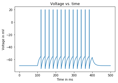
We compare this theoretical value with the average firing rates we generate from our simulations using the LIF model we constructed above. We’ll do this for several values of $I_{stim}$ , so we need to put some of the previous code (Steps 3-6) inside a for loop, iterating over different values of $I_{stim}$ . For our case, we will loop over 11 values of $I_{stim}$ from 1.43 to 1.83. The compiled code for the modified Steps 3-6 are as follows:

#Step 3: Define Initial Values and Vectors to Hold Results
t_vect = np.arange(0,t_end+dt,dt) #will hold vector of times
V_vect = np.zeros((len(t_vect),)) #initialize the voltage vector
V_plot_vect = np.zeros((len(t_vect),)) #pretty version of V_vect to be plotted that displays a spike whenever voltage reaches threshold
I_Stim_vect = np.arange(1.43,1.84,0.04) #magnitude of pulse of injected current [nA]
for j in range(len(I_Stim_vect)): #loop over different I_Stim values
	I_Stim = I_Stim_vect[j]
	V_vect[0] = E_L #value of V at t = 0
	V_plot_vect[0] = V_vect[0] #if no spike, then just plot the actual voltage V
	I_e_vect = np.zeros((len(t_vect),)) #injected current [nA]
	I_e_vect[np.int(t_StimStart/dt):np.int(t_StimEnd/dt)+1] = I_Stim*np.ones((np.int((t_StimEnd-t_StimStart)/dt)+1,))
	NumSpikes = 0 #holds number of spikes that have occurred

	#Step 4: Write Leaky Integrate-and-Fire Neuron Model
	for i in range(1,np.int(t_end/dt)+1): #loop through values of t in steps of dt ms, start with t=1 since we already defined V at t=0
		V_vect[i] = E_L + I_e_vect[i]*R_m + (V_vect[i-1] - E_L - I_e_vect[i]*R_m)*np.exp(-dt/tau)
		
		if (V_vect[i] > V_th): #neuron spiked
			V_vect[i] = V_reset #set voltage back to V_reset
			V_plot_vect[i] = V_spike #set vector that will be plotted to show a spike here
			NumSpikes += 1 #add 1 to the total spike count

		else: #voltage didn't cross threshold so neuron does not spike
			V_plot_vect[i] = V_vect[i] #plot actual voltage

	#Step 5: Make Plots
	plt.plot(t_vect, V_plot_vect)
	plt.title('Voltage vs. time')
	plt.xlabel('Time in ms')
	plt.ylabel('Voltage in mV')
	plt.show()

	#Step 6: Calculate average firing rate
	r_ave = 1000*NumSpikes/(t_StimEnd-t_StimStart) #gives average firing rate in [#/sec = Hz]
	print('Input current: ', I_Stim, 'nA')    
	print('Average firing rate: ', r_ave, 'Hz')

png

Input current:  1.43 nA
Average firing rate:  0.0 Hz

png

Input current:  1.47 nA
Average firing rate:  0.0 Hz

png

Input current:  1.51 nA
Average firing rate:  16.666666666666668 Hz

png

Input current:  1.55 nA
Average firing rate:  26.666666666666668 Hz

png

Input current:  1.59 nA
Average firing rate:  30.0 Hz

png

Input current:  1.63 nA
Average firing rate:  33.333333333333336 Hz

png

Input current:  1.67 nA
Average firing rate:  36.666666666666664 Hz

png

Input current:  1.71 nA
Average firing rate:  40.0 Hz

png

Input current:  1.75 nA
Average firing rate:  43.333333333333336 Hz

png

Input current:  1.79 nA
Average firing rate:  46.666666666666664 Hz

png

Input current:  1.83 nA
Average firing rate:  50.0 Hz

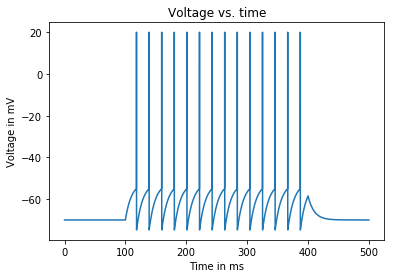
We see that as we increase the current injected into the neuron, the average firing rate also increases. We want to plot this relationship in a firing rate (Hz) vs. injected current (nA) graph. We’ll add another figure that plots the theoretical firing rate vs. I_e curve for values of $I_e$ above firing rate threshold $I_{th}$ . We’ll code this by defining a vector of injected currents $I_{vect}$ and then typing carefully the ugly formula for $r_{isi}$ from Eq4. This is defined by Step 7 below.

We only have one more modification left. We want to add onto this graph the values of $r_{ave}$ corresponding to the results of the set of simulations we generated previously. We’ll do this by converting $r_{ave}$ into a vector with the resulting average firing rates as its element.

The next block presents the final compiled code for this in silico experiment of simulating a leaky integrate-and-fire model of a neuron under a static injected current.

#Simulate a Leaky Integrate-and-Fire Neuron Model with Static Input Current

#Step 1: Import Relevant Packages
import numpy as np
import matplotlib.pyplot as plt

#Step 2: Define Parameters
dt = 0.1 #time step [ms]
t_end = 500 #total time of run [ms]
t_StimStart = 100 #time to start injecting current [ms]
t_StimEnd = 400 #time to end injecting current [ms]
E_L = -70 #resting membrane potential [mV]
V_th = -55 #spike threshold [mV]
V_reset = -75 #value to reset voltage to after a spike [mV]
V_spike = 20 #value to draw a spike to, when cell spikes [mV]
R_m = 10 #membrane resistance [MOhm]
tau = 10 #membrane time constant [ms]

#Step 3: Define Initial Values and Vectors to Hold Results
t_vect = np.arange(0,t_end+dt,dt) #will hold vector of times
V_vect = np.zeros((len(t_vect),)) #initialize the voltage vector
V_plot_vect = np.zeros((len(t_vect),)) #pretty version of V_vect to be plotted that displays a spike whenever voltage reaches threshold
I_Stim_vect = np.arange(1.43,1.84,0.04) #magnitude of pulse of injected current [nA]
r_ave_vect = np.zeros((len(I_Stim_vect),)) #vector that will hold the average firing rates for different input current values

for j in range(len(I_Stim_vect)): #loop over different I_Stim values
	
	I_Stim = I_Stim_vect[j]
	V_vect[0] = E_L #value of V at t = 0
	V_plot_vect[0] = V_vect[0] #if no spike, then just plot the actual voltage V
	I_e_vect = np.zeros((len(t_vect),)) #injected current [nA]
	I_e_vect[np.int(t_StimStart/dt):np.int(t_StimEnd/dt)+1] = I_Stim*np.ones((np.int((t_StimEnd-t_StimStart)/dt)+1,))
	NumSpikes = 0 #holds number of spikes that have occurred

	#Step 4: Write Leaky Integrate-and-Fire Neuron Model
	for i in range(1,np.int(t_end/dt)+1): #loop through values of t in steps of dt ms, start with t=1 since we already defined V at t=0
		
		V_vect[i] = E_L + I_e_vect[i]*R_m + (V_vect[i-1] - E_L - I_e_vect[i]*R_m)*np.exp(-dt/tau)
		
		if (V_vect[i] > V_th): #neuron spiked
			V_vect[i] = V_reset #set voltage back to V_reset
			V_plot_vect[i] = V_spike #set vector that will be plotted to show a spike here
			NumSpikes += 1 #add 1 to the total spike count

		else: #voltage didn't cross threshold so neuron does not spike
			V_plot_vect[i] = V_vect[i] #plot actual voltage

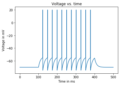
	#Step 5: Make Plots
	plt.plot(t_vect, V_plot_vect)
	plt.title('Voltage vs. time')
	plt.xlabel('Time in ms')
	plt.ylabel('Voltage in mV')
	plt.show()

	#Step 6: Calculate average firing rate
	r_ave = 1000*NumSpikes/(t_StimEnd-t_StimStart) #gives average firing rate in [#/sec = Hz]
	r_ave_vect[j] = r_ave #store the average firing rate
	print('Input current: ', I_Stim, 'nA')    
	print('Average firing rate: ', r_ave, 'Hz')

#Step 7: Compare theoretical interspike-interval firing rate with simulated average firing rate
I_th = (V_th - E_L)/R_m #neuron will not fire if the input current is below this level
I_vect = np.arange(I_th+0.001,1.8,0.001) #vector of injected current for producing theory plot
r_isi = 1000/(tau*np.log((R_m*I_vect+E_L-V_reset)/(R_m*I_vect+E_L-V_th))) #theoretical interspike-interval firing rate values
plt.plot(I_vect,r_isi)
plt.plot(I_Stim_vect,r_ave_vect,'ro')
plt.legend(['r_isi','r_ave'], loc = 'best')
plt.title('Comparison of r_isi vs. I_e and r_ave vs. I_e')
plt.xlabel('Input current [nA]')
plt.ylabel('Firing rate [Hz]')
plt.show()

png

Input current:  1.43 nA
Average firing rate:  0.0 Hz

png

Input current:  1.47 nA
Average firing rate:  0.0 Hz

png

Input current:  1.51 nA
Average firing rate:  16.666666666666668 Hz

png

Input current:  1.55 nA
Average firing rate:  26.666666666666668 Hz

png

Input current:  1.59 nA
Average firing rate:  30.0 Hz

png

Input current:  1.63 nA
Average firing rate:  33.333333333333336 Hz

png

Input current:  1.67 nA
Average firing rate:  36.666666666666664 Hz

png

Input current:  1.71 nA
Average firing rate:  40.0 Hz

png

Input current:  1.75 nA
Average firing rate:  43.333333333333336 Hz

png

Input current:  1.79 nA
Average firing rate:  46.666666666666664 Hz

png

Input current:  1.83 nA
Average firing rate:  50.0 Hz

png

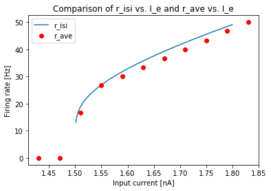
As can be seen from the graph above, the plot of average firing rates from our simulations match the theoretical firing rate curve whose formula we derived analytically. The small discrepancies are due to the difference between our experiment’s time window of counting and the total number of interspike intervals. Theoretically, if we started our time window of counting spikes for computing $r_{ave}$ when the voltage was at $V_{reset}$ (i.e. just after a spike) and ended our time window just after another spike, then these two measures should be the same. But looking at our simulations, the neuron was about to spike when we cut off the stimulus, so our $r_{ave}$ rate is smaller than $r_{isi} = 1/t_{isi}$ . Because we ended our time window just before a spike, then for a 300 ms window, this will decrease $r_{ave}$ by (1 spike)/(300 ms) = 3.33 Hz.

Now it’s your time to experiment!

Modify the code above and let’s put our thinking caps on!

Conduct simulations to find the value of the threshold current $I_{th}$ . Compare your output with the analytical value.
Can you find a time window that will make the plot of average firing rates perfectly match the theoretical firing rate curve?
Play around the relationships of the resting potential $E_L$ , threshold voltage $V_{th}$ and the reset value $V_{reset}$ . What happens if $V_{th}$ is closer to $E_L$ ? What happens if $V_{reset}$ is far smaller than $E_L$ ? What if these three values are closer to each other? farther?
What happens if we change the value of the injected current halfway through the stimulation? What if it changes four times all throughout? What if it changes continuously as a function of time?

Share on

Twitter Facebook Google+ LinkedIn

Jakov Dumbrique

Part 1: Model the subthreshold voltage dynamics

Step 1: Import Relevant Packages

Step 2: Define Parameters

Step 3: Define Initial Values and Vectors to Hold Results

Step 4: Write Leaky Integrate-and-Fire Neuron Model

Step 5: Make Plots

Part 2: Add the spiking to the model and calculate the firing rate

Step 3 (v2): Define Initial Values and Vectors to Hold Results

Step 4 (v2): Write Leaky Integrate-and-Fire Neuron Model

Step 5 (v2): Make Plots

Step 3 (v3): Define Initial Values and Vectors to Hold Results

Step 4 (v3): Write Leaky Integrate-and-Fire Neuron Model

Step 5 (v2): Make Plots

Step 6: Calculate average firing rate

Part 3: Compare theoretical firing rate vs. average firing rate

Now it’s your time to experiment!

Share on